RNA-Seq
Key Learning Outcomes
After completing this practical the trainee should be able to:
-
Understand and perform a two condition RNA-Seq expression analysis workflow.
-
Perform spliced alignments to an indexed reference genome using TopHat.
-
Visualize spliced transcript alignments in a genome browser such as IGV.
-
Be able to identify differential gene expression between two experimental conditions.
We also have bonus exercises where you can learn to:
-
Perform transcript assembly using Stringtie.
analysis.
-
Visualize transcript alignments and annotation in a genome browser such as IGV.
Author Information
Primary Author(s): Sonika Tyagi, Monash University and Susan Corley, UNSW
Contributor(s) Myrto Kostadima EBI UK
Resources You’ll be Using
Tools Used
-
Stringtie : http://https://ccb.jhu.edu/software/stringtie/
-
Samtools : http://www.htslib.org/
-
BEDTools : https://github.com/arq5x/bedtools2
-
UCSC tools : http://hgdownload.cse.ucsc.edu/admin/exe/
-
FeatureCount : http://subread.sourceforge.net/
-
edgeR pakcage : https://bioconductor.org/packages/release/bioc/html/edgeR.html
Sources of Data
http://www.ebi.ac.uk/ena/data/view/ERR022484\ http://www.ebi.ac.uk/ena/data/view/ERR022485\ http://www.pnas.org/content/suppl/2008/12/16/0807121105.DCSupplemental
Introduction
The goal of this hands-on session is to perform some basic tasks in the downstream analysis of RNA-seq data.
First we will use RNA-seq data from zebrafish. You will align one set of reads to the zebrafish using Tophat2. You will then view the aligned reads using the IGV viewer. We will also demonstrate how gene counts can be derived from this data. You will go on to assembly a transcriptome from the read data using cufflinks. We will show you how this type of data may be analysed for differential expression.
The second part of the tutorial will focus on RNA-seq data from a human experiment (cancer cell line versus normal cells). You will use the Bioconductor packages edgeR and voom (limma) to determine differential gene expression. The results from this analysis will then be used in the final session which introduces you to some of the tools used to gain biological insight into the results of a differential expression analysis
Prepare the Environment
We will use a dataset derived from sequencing of mRNA from Danio rerio
embryos in two different developmental stages. Sequencing was performed
on the Illumina platform and generated 76bp paired-end sequence data
using polyA selected RNA. Due to the time constraints of the practical
we will only use a subset of the reads.
The data files are contained in the subdirectory called data and are
the following:
2cells_1.fastq and 2cells_2.fastq
:
These files are based on RNA-seq data of a 2-cell zebrafish embryo
6h_1.fastq and 6h_2.fastq
:
These files are based on RNA-seq data of zebrafish embryos 6h post
fertilization
Open the Terminal and go to the rnaseq working directory:
cd /home/trainee/rnaseq/
All commands entered into the terminal for this tutorial should be from
within the /home/trainee/rnaseq directory.
Check that the data directory contains the above-mentioned files by
typing:
ls data
Alignment
There are numerous tools for performing short read alignment and the choice of aligner should be carefully made according to the analysis goals/requirements. Here we will use Tophat2, a widely used ultrafast aligner that performs spliced alignments.
Tophat2 is based on the Bowtie2 aligner and uses an indexed genome for
the alignment to speed up the alignment and keep its memory footprint
small. The the index for the Danio rerio genome has been created for
you.
The command to create an index is as follows. You DO NOT need to run this command yourself - we have done this for you.
STOP
DO NOT run this command. This has already been run for you.
bowtie2-build genome/Danio_rerio.Zv9.66.dna.fa genome/ZV9
Tophat2 has a number of parameters in order to perform the alignment. To view them all type:
tophat2 --help
The general format of the tophat2 command is:
tophat2 [options]* <index_base> <reads_1> <reads_2>
Where the last two arguments are the .fastq files of the paired end
reads, and the argument before is the basename of the indexed genome.
The quality values in the FASTQ files used in this hands-on session are
Phred+33 encoded. We explicitly tell tophat of this fact by using the
command line argument –solexa-quals.
You can look at the first few reads in the file data/2cells_1.fastq
with:
head -n 20 data/2cells_1.fastq
-g: Maximum number of multihits allowed. Short reads are likely to map to more than one location in the genome even though these reads can have originated from only one of these regions. In RNA-seq we allow for a limited number of multihits, and in this case we ask Tophat to report only reads that map at most onto 2 different loci.-
–library-type: Before performing any type of RNA-seq analysis you need to know a few things about the library preparation. Was it done using a strand-specific protocol or not? If yes, which strand? In our data the protocol was NOT strand specific. -
-j: Improve spliced alignment by providing Tophat with annotated splice junctions. Pre-existing genome annotation is an advantage when analysing RNA-seq data. This file contains the coordinates of annotated splice junctions from Ensembl. These are stored under the sub-directoryannotationin a file calledZV9.spliceSites. -
-o: This specifies in which subdirectory Tophat should save the output files. Given that for every run the name of the output files is the same, we specify different directories for each run.
It takes some time (approx. 20 min) to perform tophat spliced
alignments, even for this subset of reads. Therefore, we have
pre-aligned the 2cells data for you using the following command:
STOP
DO NOT run this command. This has already been run for you.
tophat2 --solexa-quals -g 2 --library-type fr-unstranded -j annotation/Danio_rerio.Zv9.66.spliceSites -o tophat/ZV9_2cells genome/ZV9 data/2cells_1.fastq data/2cells_2.fastq
Align the 6h data yourself using the following command:
    # Takes approx. 20mins
    tophat2 --solexa-quals -g 2 --library-type fr-unstranded -j annotation/Danio_rerio.Zv9.66.spliceSites -o tophat/ZV9_6h genome/ZV9 data/6h_1.fastq data/6h_2.fastq
The 6h read alignment will take approx. 20 min to complete. Therefore,
we’ll take a look at some of the files, generated by tophat, for the
pre-computed 2cells data.
Tophat generates several files in the specified output directory. The most important files are listed below.
accepted_hits.bam
: This file contains the list of read alignments in BAM format.
align_summary.txt
: Provides a detailed summary of the read-alignments.
unmapped.bam
: This file contains the unmapped reads.
The complete documentation can be found at: https://ccb.jhu.edu/software/tophat/manual.shtml
Alignment Visualisation in IGV
The Integrative Genomics Viewer (IGV) is able to provide a visualisation
of read alignments given a reference sequence and a BAM file. We’ll
visualise the information contained in the accepted_hits.bam and
junctions.bed files for the pre-computed 2cells data. The former,
contains the tophat spliced alignments of the reads to the reference
while the latter stores the coordinates of the splice junctions present
in the data set.
Open the rnaseq directory on your Desktop and double-click the
tophat subdirectory and then the ZV9_2cells directory.
-
Launch IGV by double-clicking the “IGV 2.3.*” icon on the Desktop (ignore any warnings that you may get as it opens).
NOTE: IGV may take several minutes to load for the first time, please be patient.
-
Choose “Zebrafish (Zv9)” from the drop-down box in the top left of the IGV window. Else you can also load the genome fasta file.
-
Load the
accepted_hits.sorted.bamfile by clicking the “File” menu, selecting “Load from File” and navigating to theDesktop/rnaseq/tophat/ZV9_2cellsdirectory. -
Rename the track by right-clicking on its name and choosing “Rename Track”. Give it a meaningful name like “2cells BAM”.
-
Load the
junctions.bedfrom the same directory and rename the track “2cells Junctions BED”. -
Load the Ensembl annotations file
Danio_rerio.Zv9.66.gtfstored in thernaseq/annotationdirectory. -
Navigate to a region on chromosome 12 by typing
chr12:20,270,921-20,300,943into the search box at the top of the IGV window.
Keep zooming to view the bam file alignments
Some useful IGV manuals can be found below
http://www.broadinstitute.org/software/igv/interpreting_insert_size\ http://www.broadinstitute.org/software/igv/alignmentdata
Does the file ’align_summary.txt’ look interesting? What information does it provide?
As the name suggests, the file provides a details summary of the alignment statistics.
One other important file is ’unmapped.bam’. This file contains the unampped reads.
Can you identify the splice junctions from the BAM file?
Splice junctions can be identified in the alignment BAM files. These are the aligned RNA-Seq reads that have skipped-bases from the reference genome (most likely introns).
Are the junctions annotated for CBY1 consistent with the annotation?
Read alignment supports an extended length in exon 5 to the gene model (cby1-001)
Once tophat finishes aligning the 6h data you will need to sort the alignments found in the BAM file and then index the sorted BAM file.
samtools sort tophat/ZV9_6h/accepted_hits.bam -o tophat/ZV9_6h/accepted_hits.sorted.bam
samtools index tophat/ZV9_6h/accepted_hits.sorted.bam
Load the sorted BAM file into IGV, as described previously, and rename the track appropriately.
Generating Gene Counts
In RNAseq experiments the digital gene expression is recorded as the
gene counts or number of reads aligning to a known gene feature. If you
have a well annotated genome, you can use the gene structure file in a
standard gene annotation format (GTF or GFF)) along with the spliced
alignment file to quantify the known genes. We will demonstrate a
utility called FeatureCounts that comes with the Subread package.
mkdir gene_counts
featureCounts -a annotation/Danio_rerio.Zv9.66.gtf -t exon -g gene_id -o gene_counts/gene_counts.txt tophat/ZV9_6h/accepted_hits.sorted.bam tophat/ZV9_2cells/accepted_hits.sorted.bam
Isoform Expression and Transcriptome Assembly
For non-model organisms and genomes with draft assemblies and incomplete
annotations, it is a common practice to take and assembly based approach
to generate gene structures followed by the quantification step. There
are a number of reference based transcript assemblers available that can
be used for this purpose such as, cufflinks, stringtie. These assemblers
can give gene or isoform level assemblies that can be used to perform a
gene/isoform level quantification. These assemblers require an alignment
of reads with a reference genome or transcriptome as an input. The
second optional input is a known gene structure in GTF or GFF
format.
These gene annotation files contain information of known genes and may be helpful in reconstruction of transcripts that are of low abundance on your sample. StringTie will also assemble and construct a transcriptome containing any unannotated genes. Furthermore, its output data is able to directly be utilised in differential expression resources such as Cuffdiff, Ballgown or other packers in R (edgeR, DESeq2).
To run string tie, the basic command is:
Stringtie has a number of parameters in order to perform transcriptome assembly and quantification. To view them all type:
stringtie --help
The Ensembl annotation for Danio rerio is available in
annotation/Danio_rerio.Zv9.66.gtf.
The general format of the stringtie command is:
stringtie <aligned_reads_file.bam> [options]
Perform transcriptome assembly, strictly using the supplied GTF
annotations, for the 2cells and 6h data using cufflinks:
For instance, to run StringTie on 2cells BAM file:
stringtie -p 8 -G annotation/Danio_rerio.Zv9.66.gtf -o stringtie/ZV9_2cells.gtf tophat/ZV9_2cells/accepted_hits.sorted.bam
Repeat this command on the 6h BAM file:
stringtie -p 8 -G annotation/Danio_rerio.Zv9.66.gtf -o stringtie/ZV9_6h.gft tophat/ZV9_6h/accepted_hits.sorted.bam
-
-p= number of processing threads -
-G= reference annotation file -
-o= output file location and name.
Most RNA sequencing experiments will have multiple samples. As such, Stringtie has a function to merge all transcripts assembled across the samples, which enables inter-sample comparisons to be made. It does this by first assembling all transcripts within each sample, merging the the transcripts and re-running the assembly based off a merged list of genes.
Prior to running a merge function within stringtie: We need to create a mergelist.txt file before utilising the merge function. This is a list of all .gtf files created by stringtie in the above step and can be made in a text editor such as vi or nano. For this exercise, there is a file pre-made for you. The txt file will direct the merge function to look for the names of all the .gtf files that we want to merge.
To merge StringTie files
    ls stringtie/*.gtf >mergelist.txt
    less mergelist.txt

    stringtie --merge -p 8 -G annotation/Danio_rerio.Zv9.66.gtf -o stringtie/stringtie_merged.gtf mergelist.txt
mergelist.txt is a text file that will have a list of all .gtf generated by stringtie in the above steps)
Note how a reference gene annotation (Danio_rerio.Zv9.66.gtf) is utilised in this case. This makes use of information we already have in order to assemble the transcriptome of our RNA seq data.
The next step is an optional step to see how your merged annotation compares to reference gene annotation provided. gffcompare is a tool that determines how many of your annotations match the reference (either fully or partial) and how many were completely novel. The output of this ulitily gives you:
Sensitivity is defined as the proportion of genes from the annotation that are correctly reconstructed Precision (also known as positive predictive value) captures the proportion of the output that overlaps the annotation To compare how merged annotation compares to reference
gffcompare -G -r annotation/Danio_rerio.Zv9.66.gtf stringtie/stringtie_merged.gtf
-
-r = reference genome in form of gtf
-
-G = tells gffcompare to compare all transcripts in the input file (stringtie/stringtie_merged.gtf), even those that might be redundant
-
-o = all output of gffcompare has a gffcmp. prefix, unless otherwise defined by user
Now that we are happy with our merged annotation, we need to estimate the abundance of each transcript within each sample. Stringtie is designed to create output files that are immediately usable in next step of our RNA sequencing pipeline. In this next example, we can direct stringtie to simultaneously create a .ctab file required for ballgown.
To estimate abundances and create table counts for 2cell
stringtie -e -B -p 8 -G stringtie/stringtie_merged.gtf -o ballgown/ZV9_6h.gtf tophat/ZV9_6h/accepted_hits.sorted.bam
stringtie -e -B -p 8 -G stringtie/stringtie_merged.gtf -o ballgown/ZV9_2cells.gtf tophat/ZV9_2cells/accepted_hits.sorted.bam
-
-e = limits the processing of read alignments to only estimate and output the assembled transcripts matching the reference transcripts (given by -G). Reads with no reference transcripts will be entirely skipped
-
-B = enables output of Ballgown input table files (*.ctab) containing coverage data for the reference transcripts given with the -G option. If -o is used, StringTie will write the *.ctab files in the same directory as the output GTF.
-
-p = refers to number of processing threads
-
-G = refers to a reference annotation (in GTF or GFF format)
Visulaizing transcript assembly
-
Go back to IGV and load the pre-computed, GTF-guided transcriptome assembly for the
2cellsdata (stringtie/ZV9_2cells.gtf). -
Rename the track as “2cells GTF-Guided Transcripts”.
-
In the search box type
ENSDART00000082297in order for the browser to zoom in to the gene of interest.
Do you observe any difference between the Ensembl GTF annotations and the GTF-guided transcripts assembled by cufflinks (the “2cells GTF-Guided Transcripts” track)?
Yes. It appears that the Ensembl annotations may have truncated the last exon. However, our data also doesn’t contain reads that span between the last two exons.
Differential Gene Expression Analysis using edgeR
Experiment Design
The example we are working through today follows a case Study set out in the edgeR Users Guide (4.3 Androgen-treated prostate cancer cells (RNA-Seq, two groups) which is based on an experiment conducted by Li et al. (2008, Proc Natl Acad Sci USA, 105, 20179-84).
The researches used a prostate cancer cell line (LNCaP cells). These cells are sensitive to stimulation by male hormones (androgens). Three replicate RNA samples were collected from LNCaP cells treated with an androgen hormone (DHT). Four replicates were collected from cells treated with an inactive compound. Each of the seven samples was run on a lane (7 lanes) of an Illumina flow cell to produce 35 bp reads. The experimental design was therefore:
| Lane | Treatment | Label |
|---|---|---|
| 1 | Control | Con1 |
| 2 | Control | Con2 |
| 3 | Control | Con3 |
| 4 | Control | Con4 |
| 5 | DHT | DHT1 |
| 6 | DHT | DHT2 |
| 7 | DHT | DHT3 |
This workflow requires raw gene count files and these can be generated
using a utility called featureCounts as demonstrated above. We are using
a pre-computed gene counts data (stored in pnas_expression.txt) for
this exercise.
Prepare the Environment
Prepare the environment and load R:
    cd /home/trainee/rnaseq/edgeR
    R (press enter)
    library(edgeR)
    library(biomaRt)
    library(gplots)
    library("limma")
    library("RColorBrewer")
    library("org.Hs.eg.db")
Read in Data
Read in count table and experimental design:
    data <- read.delim("pnas_expression.txt", row.names=1, header=T)
    targets <- read.delim("Targets.txt", header=T)
    colnames(data) <-targets$Label
    head(data, n=20)
Add Gene annotation
The data set only includes the Ensembl gene id and the counts. It is useful to have other annotations such as the gene symbol and entrez id. Next we will add in these annotations. We will use the BiomaRt package to do this.
We start by using the useMart function of BiomaRt to access the human data base of ensemble gene ids.
    human<-useMart(host="www.ensembl.org", "ENSEMBL_MART_ENSEMBL", dataset="hsapiens_gene_ensembl")
    attributes=c("ensembl_gene_id", "entrezgene_id","hgnc_symbol")
    ensembl_names<-rownames(data)
    head(ensembl_names)
genemap<-getBM(attributes, filters="ensembl_gene_id", values=ensembl_names, mart=human)
head(genemap)
    idx <-match(ensembl_names, genemap$ensembl_gene_id)
    data$entrezgene <-genemap$entrezgene_id [ idx ]
    data$hgnc_symbol <-genemap$hgnc_symbol [ idx ]
    Ann <- cbind(rownames(data), data$hgnc_symbol, data$entrezgene)
    colnames(Ann)<-c("Ensembl", "Symbol", "Entrez")
    Ann<-as.data.frame(Ann)
head(data)
Data checks
Create DGEList object:
    treatment <-factor(c(rep("Control",4), rep("DHT",3)), levels=c("Control", "DHT"))
    y <-DGEList(counts=data[,1:7], group=treatment, genes=Ann)
dim(y)
Now we will filter out genes with low counts by only keeping those rows where the count per million (cpm) is at least 1 in at least three samples:
# Here we calculate the number of counts per million (cpm) reads as a normalization factor
myCPM <- cpm(y$counts)
dim(myCPM)

# Here we generate a graph and save it as a pdf comparing raw counts with cpm
# we want to remove all those genes that have too low counts which may be due to noise

pdf(file="counts-vs-cpms-gene.pdf")
plot(myCPM[,1],y$counts[,1],ylim=c(0,30),xlim=c(0,3))
for (i in 1:3) {
  abline(h=10,v=i)
  i<-i+1
}
dev.off()


head(myCPM)
thresh <- myCPM > 1 ## we selected a threshold of at least 1 cpm on each gene on each sample
head(thresh)
table(rowSums(thresh))

# we would like to keep genes that have at least 2 TRUES, two samples with more than 1 cpm in each row (gene).

keep <- rowSums(thresh) >=3

y$counts<-y$counts[keep,]

# dim function will tell us the number of genes that we kept with high enough expression

dim(y$counts)
Question
Hint
dim(y)
Answer
16494
Question
Hint
do 37435-16494.
As we have removed the lowly expressed genes the total number of counts per sample has not changed greatly. Let us check the total number of reads per sample in the original data (data) and now after filtering.
Before:
colSums(data[,1:7])
colSums(y$counts)
y<-calcNormFactors(y)
y$samples
plotMDS(y, col=as.numeric(y$samples$group))
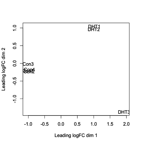 [fig:MDS plot]
Does the MDS plot indicate a difference in gene expression between the Controls and the DHT treated samples?
The MDS plot shows us that the controls are separated from the DHT treated cells. This indicates that there is a difference in gene expression between the conditions.
We will now estimate the dispersion. We start by estimating the common dispersion. The common dispersion estimates the overall Biological Coefficient of Variation (BCV) of the dataset averaged over all genes.
By using verbose we get the Disp and BCV values printed on the screen
y <- estimateCommonDisp(y, verbose=T)
We now estimate gene-specific dispersion.
y <- estimateTagwiseDisp(y)
plotBCV(y)
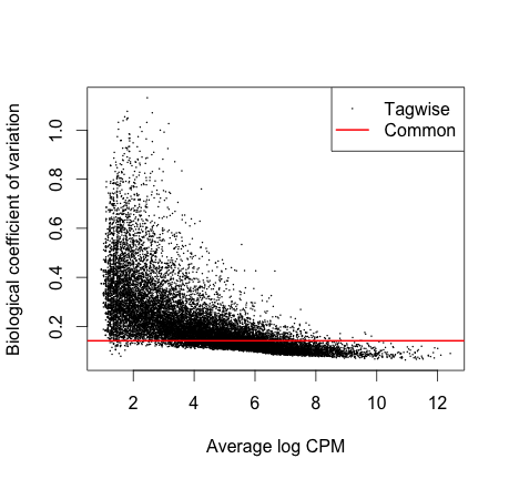 [fig:BCV plot]
We see here that the common dispersion estimates the overall Biological
Coefficient of Variation (BCV) of the dataset averaged over all genes.
The common dispersion is 0.02 and the BCV is the square root of the
common dispersion (sqrt[0.02] = 0.14). A BCV of 14% is typical for cell
line experiment.
As you can see from the plot the BCV of some genes (generally those with low expression) can be much higher than the common dispersion. For example we see genes with a reasonable level of expression with tagwise dispersion of 0.4 indicating 40% variation between samples.
If we used the common dispersion for these genes instead of the tagwise dispersion what effect would this have?
If we simply used the common dispersion for these genes we would underestimate biological variability, which in turn affects whether these genes would be identified as being differentially expressed between conditions.It is recommended to use the tagwise dispersion, which takes account of gene-to-gene variability.
Now that we have normalized our data and also calculated the variability of gene expression between samples we are in a position to perform differential expression testing.As this is a simple comparison between two conditions, androgen treatment and placebo treatment we can use the exact test for the negative binomial distribution (Robinson and Smyth, 2008).
Testing for Differential Expression
We now test for differentially expressed BCV genes:
et <- exactTest(y)
res <- topTags(et, n=nrow(y$counts), adjust.method="BH")$table
head(res)
summary(de <- decideTestsDGE(et))
    alpha=0.05
    lfc=1.5
    edgeR_res_sig<-res[res$FDR<alpha,]
    edgeR_res_sig_lfc <-edgeR_res_sig[abs(edgeR_res_sig$logFC) >= lfc,]
    head(edgeR_res_sig, n=20)nrow(edgeR_res_sig)nrow(edgeR_res_sig_lfc)
Question
How many differentially expressed genes are there?
Answer
4435
Question
Answer
2339 2096
If you need to quit the R console, type:
q()
You can save your workspace by typing Y on prompt.
Please note that the output files you are creating are saved in your
present working directory. If you are not sure where you are in the file
system try typing pwd on your command prompt to find out.
References
-
Trapnell, C., Pachter, L. & Salzberg, S. L. TopHat: discovering splice junctions with RNA-Seq. Bioinformatics 25, 1105-1111 (2009).
-
Trapnell, C. et al. Transcript assembly and quantification by RNA-Seq reveals unannotated transcripts and isoform switching during cell differentiation. Nat. Biotechnol. 28, 511-515 (2010).
-
Langmead, B., Trapnell, C., Pop, M. & Salzberg, S. L. Ultrafast and memory-efficient alignment of short DNA sequences to the human genome. Genome Biol. 10, R25 (2009).
-
Roberts, A., Pimentel, H., Trapnell, C. & Pachter, L. Identification of novel transcripts in annotated genomes using RNA-Seq. Bioinformatics 27, 2325-2329 (2011).
-
Roberts, A., Trapnell, C., Donaghey, J., Rinn, J. L. & Pachter, L. Improving RNA-Seq expression estimates by correcting for fragment bias. Genome Biol. 12, R22 (2011).
-
Robinson MD, McCarthy DJ and Smyth GK. edgeR: a Bioconductor package for differential expression analysis of digital gene expression data. Bioinformatics, 26 (2010).
-
Robinson MD and Smyth GK Moderated statistical tests for assessing differences in tag abundance. Bioinformatics, 23, pp. -6.
-
Robinson MD and Smyth GK (2008). Small-sample estimation of negative binomial dispersion, with applications to SAGE data.” Biostatistics, 9.
-
McCarthy, J. D, Chen, Yunshun, Smyth and K. G (2012). Differential expression analysis of multifactor RNA-Seq experiments with respect to biological variation. Nucleic Acids Research, 40(10), pp. -9.